Halloween Candy
This data comes from the candy hierarchy data which was published annually around Halloween from 2014 to 2017. I used the 2015, 2016 and 2017 data sets. The raw data for 2014 is not available and so I did not include it.
The data was generated from an online survey of thousands of people from around the world, assessing their joy, despair or ambivalence to a wide range of Halloween candy and non-candy items.
There are a lot of free text columns and a range of auxiliary non-candy related questions in the survey. The main goal of this project was to gain experience cleaning and wrangling a real world data set. And oh how the halloween candy delivered on this! However this did mean that I didn’t have much time to explore and visualise the data. So now I will take a closer look.
Data cleaning
The full cleaning scripts can be found in my GitHub repository.
Summary of the steps taken to clean the data:
- column names cleaned
- columns were selected based on downstream analyses required in the brief
- missing values were corrected or recoded where possible, otherwise they were left in the data
- the country column was recoded to US, UK, Canada or Other
- the three datasets were transformed from wide to long format
- age was limited to reasonable values
- a confectionery column was added to select conventional candy for analyses
- the column selection and age limiting were common tasks across all three datasets. Therefore these were written as functions in a separate functions file
Assumptions
I made a number of assumptions when wrangling the data. Two of the more important are:
- I assumed that there was a data entry issue for the country column in 2016 and 2017. There were numbers entered into the country column where the corresponding age column was empty. I transferred these to the age column.
- I also assumed that the list of candy bars provided by the survey was exhaustive. I know this cannot be the case. I will assume that they include the most popular candy bars from the UK, US and Canada.
Analysis
Exploratory Data Analysis
How many candy ratings have been given?
A total of 772352 candy ratings have been given over the three years. This is for all “candy” offered by the survey, including candy which is not a sweet. Breaking this down, 606609 ratings were given for candy you would find in a sweet shop and only 165743 ratings given for the inedible kind of candy.
What is the demographic of people completing the survey?
clean_candy %>%
  filter(!is.na(going_trick_or_treat)) %>%
  ggplot() +
  aes(x = age, fill = going_trick_or_treat) +
  geom_histogram(col = "white", bins = 40)  +
  scale_fill_discrete_qualitative(
    palette = "set 3", nmax = 5, order = c(4, 1)) +
  scale_x_continuous(breaks = seq(from = 0, to = 80, by = 10)) +
  theme +
  labs(
    title = "What is the age range of survey takers?\n",
    x = "Age",
    y = "Total number\n",
    fill = "Going trick or\n treating?"
  )

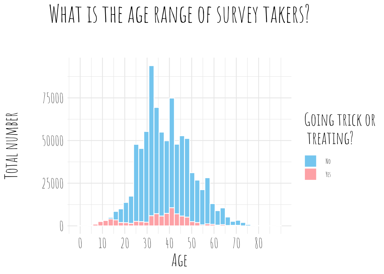
The majority of surveyed individuals were not even going trick or treating! And the average age was overwhelmingly over eighteen sitting between 25 and 50 years old. For those going trick or treating there are two peaks in the age distribution, one around 13 and the other around 35.
Does candy you can eat give you more joy?
clean_candy %>%
  filter(!is.na(joy_induction)) %>%
  mutate(confectionery = if_else(confectionery == TRUE, "Yes", "No")) %>%
  ggplot() +
  aes(x = confectionery, fill = joy_induction) +
  geom_bar(position = "fill") +
  scale_fill_discrete_qualitative(
    palette = "set 3", nmax = 5, order = c(5, 1, 2)) +
  theme +
  labs(
    title = "Satisfaction gained from edible and inedible candy\n",
    x = "Is it candy you can eat?",
    y = "Proportion of responses\n",
    fill = "Response"
  )

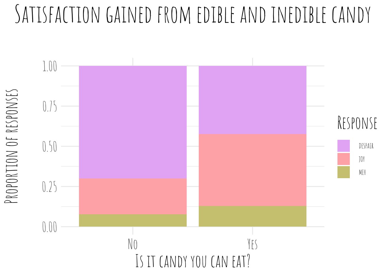
If you can eat the candy, it does seem to bring more joy. The meh rating is also higher in edible candy and the despair rating is much lower.
Just how bad were the inedible candy ratings?
To quantify the ratings, I will count despair as -1, joy as +1 and meh as 0.
rated_clean_candy <- clean_candy %>%
  mutate(
    rating = case_when(
      joy_induction == "DESPAIR" ~ as.numeric(-1),
      joy_induction == "JOY" ~ as.numeric(1),
      joy_induction == "MEH" ~ as.numeric(0),
      TRUE ~ NA_real_
    )
  )
rated_clean_candy %>%
  filter(confectionery == FALSE) %>%
  group_by(candy) %>%
  summarise(total_ratings = sum(rating, na.rm = TRUE)) %>%
  ggplot() +
  aes(x = total_ratings, y = reorder(candy, -total_ratings), fill =(total_ratings>0)) +
  geom_col() +
  scale_fill_discrete_qualitative(
    palette = "set 3", nmax = 5, order = c(1, 3)) +
  theme_2 +
  theme(legend.position = "none") +
  labs(
    title = "What did inedible candy rate?",
    x = "Total ratings",
    y = "Inedible candy\n"
  )

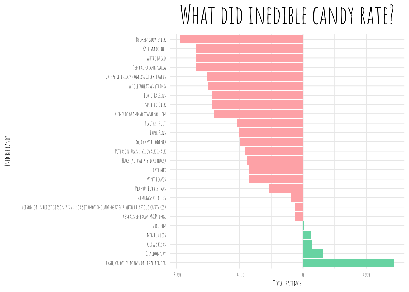
The worst inedible candy are broken glow sticks closely followed by kale smoothies (inedible in my opition!) and white bread (also not candy!).
What was the most popular candy bar in each year?
rated_clean_candy %>%
  filter(confectionery == TRUE) %>%
  select(year, candy, rating) %>%
  group_by(year, candy) %>%
  summarise(total_ratings = sum(rating, na.rm = TRUE)) %>%
  slice_max(total_ratings)
## # A tibble: 3 x 3
## # Groups:   year [3]
##    year candy                    total_ratings
##   <dbl> <chr>                            <dbl>
## 1  2015 Any full-sized candy bar          4603
## 2  2016 Any full-sized candy bar          1037
## 3  2017 Any full-sized candy bar          1542
For all three years, “Any full-sized candy bar” was the most popular candy. To find the most popular branded bar, I will filter this candy out from the data and rerun it.
rated_clean_candy %>%
  filter(confectionery == TRUE,
         candy != "Any full-sized candy bar") %>%
  select(year, candy, rating) %>%
  group_by(year, candy) %>%
  summarise(total_ratings = sum(rating, na.rm = TRUE)) %>%
  slice_max(total_ratings)
## # A tibble: 3 x 3
## # Groups:   year [3]
##    year candy                      total_ratings
##   <dbl> <chr>                              <dbl>
## 1  2015 Reese’s Peanut Butter Cups          4375
## 2  2016 Kit Kat                              920
## 3  2017 Reese’s Peanut Butter Cups          1403
The most popular branded candy bar was Reese’s Peanut Butter Cups in 2015 and 2017 and Kit Kat in 2016.
What was the most popular candy bar by this rating for people in US, Canada, UK and all other countries?
To find the best scoring branded bar, filter out the “Any full-sized candy bar” chocolate.
## # A tibble: 4 x 3
## # Groups:   country [4]
##   country candy                      total_ratings
##   <chr>   <chr>                              <dbl>
## 1 canada  Kit Kat                              231
## 2 other   Kit Kat                               58
## 3 uk      Lindt Truffle                         36
## 4 us      Reese’s Peanut Butter Cups          1983
Now we can see a clear divide in the countries favourite candy bars. Canada and the rest of the world prefer Kit Kat with a rating of 231 and 58. The UK prefers Lindt Truffle with a score of 36 and the US prefers Reese’s Peanut Butter Cups with a score of 1983.
Other interesting analyses or conclusions
What about M&M’s? Let’s have a look at what the most popular M&M types are for each country.
rated_clean_candy %>%
  mutate(
    m_n_m = if_else(str_detect(candy, "M&M"), TRUE, FALSE)) %>%
  filter(confectionery == TRUE,
         country != is.na(country),
         candy != "Any full-sized candy bar",
         m_n_m == TRUE) %>%
  select(country, candy, rating) %>%
  group_by(country, candy) %>%
  summarise(total_ratings = sum(rating, na.rm = TRUE)) %>%
  slice_max(total_ratings)
## # A tibble: 4 x 3
## # Groups:   country [4]
##   country candy        total_ratings
##   <chr>   <chr>                <dbl>
## 1 canada  Regular M&Ms           172
## 2 other   Peanut M&M’s            53
## 3 uk      Regular M&Ms            27
## 4 us      Peanut M&M’s          1645
It’s a debate between regular and peanut M&M’s. Canada and the UK rate regular M&M’s the highest with ratings of 172 and 27 respectively. The US and the rest of the world rate Peanut M&M’s the highest with ratings of 1645 and 53.
It may be worth revisiting my earlier assumption that spliting the M&M’s and the Smarties were fine for this dataset. It would be interesting to see what all M&M’s combined score.